Numerical Solution of the Falkner - Skan Equation
Falkner - Skan equation is a third order non-linear ordinary differential equation which arises in the laminar boundary layer flow past wedge-like objects. (More details here). The equation reads,
$ f’’’+\frac{m+1}{2}f f’'+m\left[1-(f’)^2\right]= 0 $
where m is a constant representing the pressure gradient parameter. Our objective is to solve this differential equation for $ f(\eta)$ , for a given value of m using the boundary conditions,
$ f(0)=0 \quad \rightarrow \text{no wall transpiration}$
$ f’(0)=0 \quad \rightarrow \text{ no-slip condition at the wall}$
$ f’(1)=1 \, \rightarrow \text{free-stream velocity is reached at the edge of the boundary layer}$
Generally, initial value problems (IVP) are preferred for ODEs. In the case of IVP, We will be given where to start and which direction to proceed. Then we use the differential equation to progress in that direction in a step by step manner. But here we have a boundary value problem. Shooting method is used in situations where a boundary value problem has to be solved using initial value methods. The method is described as follows.
Shooting method
-
Guess two values for $ f’'(0)$.
-
Solve the FS equation using RK4 method with initial conditions $ f(0)=0, f’(0)=0, f’'(0) = Guess1$.
-
Solve the FS equation using RK4 method with initial conditions $ f(0)=0, f’(0)=0, f’'(0) = Guess2$.
-
Find out the resulting boundary value $ f’(1)$ from both these solutions.
-
If the boundary value $ f’(1)$ is different from the required value $ f’(1)=1$, find a better initial guess using Secant method.
-
Solve the FS equation by RK4 method using the new initial value guess (obtained from secant method).
-
Repeat the process until the required boundary value $ f’(1)$ is obtained.
A Fortran program for solving the Falkner-Skan equation implementing the above algorithm is provided below. (Click on any part of the code and use right arrow key to scroll to right).
program falkner_skan
! this program solves the Falkner-Skan equation using shooting method and fourth order Runge-Kutta method.
! the FS equation is given by,
! f'''+((m+1)/2)ff''+ m*(1-f'^2) = 0
! m,the pressure gradient parameter, as in u_inf=u0*x^m.
! boundary conditions: f(0)=0, f'(0)=0, f'(1)=1
! the third order ode is converted into a system of three first order odes where the
! dependent variables are f, u (=f'), v (=u'=f'').
! we solve the initial value problem f(0)=0,f'(0)=0, f''(0)=guess and shoot for solutions such that f'(1)=1.
implicit none
integer :: i,j,np,niter
real,allocatable,dimension(:) :: f,u,v,eta
real :: m,mh,re,ue,f0,u0,v0,deta,x,eps,cnu,slope,unp,unp1,vnp,vnp1
real,allocatable,dimension(:) :: vvel,y,vvel1
real :: delta_star_temp,theta_temp,deltas,theta
niter=1000 ! no. of iterations for the shooting method
deta=0.001 ! non-dimensional spacing in the wall-normal direction
np=8001 ! no. of points in the wall-normal direction
eps=1.0e-16 ! error margin used in shooting method iteration
m=0.0 ! falkner-skan pressure gradient parameter
mh=0.5*(m+1.0)
allocate(f(np),u(np),v(np),eta(np),vvel(np),vvel1(np),y(np))
! form the grid in the wall-normal direction
eta(1)=0.0
do j=2,np
eta(j)=eta(j-1)+deta
enddo
! initial values set 1
f0=0.0
u0=0.0
v0=0.335
call rk4_fs(f,u,v,deta,mh,m,np,f0,u0,v0)
vnp=v(1)
unp=u(np)
! initial values set 2
f0=0.0
u0=0.0
v0=0.33
call rk4_fs(f,u,v,deta,mh,m,np,f0,u0,v0)
vnp1=v(1)
unp1=u(np)
! loop for the shooting method ********************************************************************
do i=1,niter
if (abs(unp1-1.0) .ge. eps) then
slope=(vnp1-vnp)/(unp1-unp)
v0=vnp1+slope*(1.0-unp1)
unp=unp1
vnp=vnp1
call rk4_fs(f,u,v,deta,mh,m,np,f0,u0,v0)
vnp1=v(1)
unp1=u(np)
else
write(*,*) 'iteration converged'
write(*,*) 'v(1)=',v(1)
exit
endif
if(i .eq. niter) then
write(*,*) 'maximum number of iterations reached'
endif
enddo
! end of shooting method **************************************************************************
do j=1,np
write(38,*) eta(j),f(j),u(j),v(j) ! these are transformed variables - input for box method
enddo
! calculation of normal velocity component profile
x=0.1
u0=1.0
ue=u0*(x**m)
cnu=15.0e-06
re=ue*x/cnu
do j=1,np
y(j)=eta(j)*sqrt(cnu*x/ue) ! distance from the wall in meters
vvel(j)=-((m-1.0)*eta(j)*u(j)+(m+1.0)*f(j))*(0.5/sqrt(re)) ! vvel=v/u_inf
write(48,*) eta(j),u(j),vvel(j),y(j),u(j)*ue,vvel(j)*sqrt(re)
enddo
! calculation of boundary layer parameters
theta_temp = 0.0
delta_star_temp = 0.0
do i = 1,(np-1)
theta_temp = theta_temp + 0.5*(eta(i+1)-eta(i))*(u(i+1)*(1.0-u(i+1)) + u(i)*(1.0-u(i)) )
delta_star_temp = delta_star_temp + 0.5*(eta(i+1)-eta(i))*((1.0-u(i+1))+(1.0-u(i)))
enddo
deltas=delta_star_temp*x/sqrt(re)
theta=theta_temp*x/sqrt(re)
write(*,*) '************************************************************************'
write(*,*) 'Solution of the Falkner-Skan equation'
write(*,*) '************************************************************************'
write(*,'(a,f8.5)') 'pressure gradient parameter, m=',m
write(*,'(a,f8.5,a)') 'distance from the leading edge, x=',x,' m'
write(*,'(a,f8.2)') 'Re = u_inf*x/cnu = ',re
write(*,'(a,f8.5,a)') 'displacement thickness, delta*=',deltas,' m'
write(*,'(a,f8.5,a)') 'momentum thickness, theta=',theta,' m'
write(*,*) '************************************************************************'
call system('gnuplot -p FS.plt')
return
end program falkner_skan
subroutine rk4_fs(f,u,v,deta,mh,m,np,f0,u0,v0)
! subroutine for solving a system of three first order odes with fourth order Runge-Kutta method
! f0,u0,v0 are the initial values
! f,u,v arrays give the solution
! initial values are propagated to np steps using step spacing deta.
integer :: j
real :: kf(4),ku(4),kv(4)
real,intent(in) :: m,mh,deta,f0,u0,v0
integer,intent(in) :: np
real :: f(np),u(np),v(np)
f(1)=f0
u(1)=u0
v(1)=v0
do j=2,np
ku(1)=v(j-1)
kf(1)=u(j-1)
kv(1)=-mh*f(j-1)*v(j-1)-m*(1.0-u(j-1)*u(j-1))
ku(2)=v(j-1)+0.5*kv(1)*deta
kf(2)=u(j-1)+0.5*ku(1)*deta
kv(2)=-mh*(f(j-1)+0.5*kf(1)*deta)*(v(j-1)+0.5*kv(1)*deta)-m*(1.0-(u(j-1)+0.5*ku(1)*deta)**2)
ku(3)=v(j-1)+0.5*kv(2)*deta
kf(3)=u(j-1)+0.5*ku(2)*deta
kv(3)=-mh*(f(j-1)+0.5*kf(2)*deta)*(v(j-1)+0.5*kv(2)*deta)-m*(1.0-(u(j-1)+0.5*ku(2)*deta)**2)
ku(4)=v(j-1)+kv(3)*deta
kf(4)=u(j-1)+ku(3)*deta
kv(4)=-mh*(f(j-1)+kf(3)*deta)*(v(j-1)+kv(3)*deta)-m*(1.0-(u(j-1)+ku(3)*deta)**2)
f(j)=f(j-1)+(1.0/6.0)*deta*(kf(1)+2.0*kf(2)+2.0*kf(3)+kf(4))
u(j)=u(j-1)+(1.0/6.0)*deta*(ku(1)+2.0*ku(2)+2.0*ku(3)+ku(4))
v(j)=v(j-1)+(1.0/6.0)*deta*(kv(1)+2.0*kv(2)+2.0*kv(3)+kv(4))
enddo
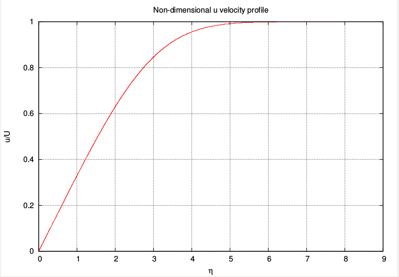
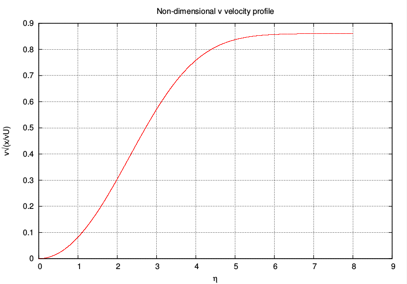
end subroutine rk4_fsLine 114 in the above code calls the gnuplot program FS.plt to plot the solution. The most relevant plots for fluid dynamics in this problem are the streamwise velocity profile $ f’(\eta)$ and the wall-normal velocity profile given by,
$ \frac{v}{U}=-\frac{1}{2\sqrt{Re_x}}\left[ (m+1)f+(m-1)\eta f’ \right] $
Sample results for the case m=0 (Blasius boundary layer) are shown below.