What is the Fourier transform?
Previous article: 1. Fourier transform for confused engineers
What is the Fourier transform, really?
For some, it is the magic of seeing everything as waves. For others, it is like holding a prism in a beam of sunlight and seeing what it contains, a rainbow of colors. For some others, it is a tool to visualize what a piece of sound recording contains and adjusting it to make it sound better.
One can even take the romanticism out of the concept and say, it converts a bunch of given numbers into another bunch. It is through doing this that many important uses of Fourier transform can be realized. And this is precisely where many miss the woods for the trees. I hope to bridge both sides of this amazing idea. Let us begin!
When we have a clearly defined function, as shown in the plot below, everything is straightforward.
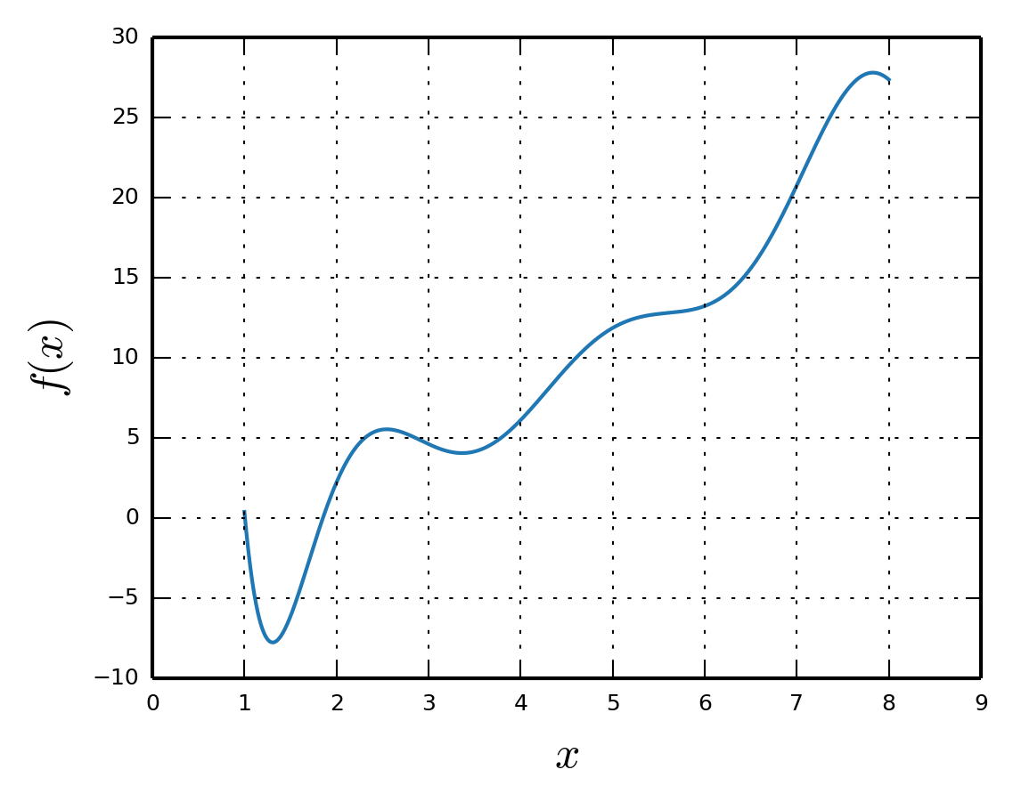
This means that we have a known expression for how the function depends on the variable x:
All the nice definitions of the Fourier transform become useful and if the integral is not monstrous, we would have a good looking expression for the Fourier transform of the function. Life is tricky and usually we only have some values of the function at hand. Like:
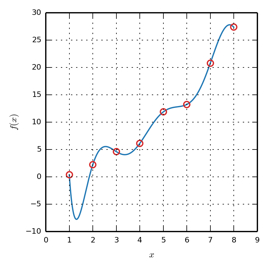
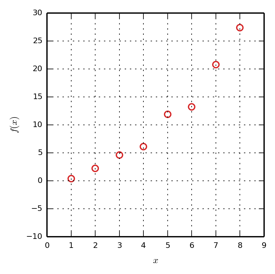
Most of the time, we just have the data points as shown by the red dots. You can imagine a function passing through the data like the blue line. But it does not matter. Now, it is just us and the red dots. The entire business of discrete Fourier transform (DFT) is to take the Fourier transform of such a bunch of data points. Before I throw some formulas at you, there are some ground rules to cover.
-
The universe plays the game strict and fair. If you have $N$ values in the data set, you will only get back $N$ number of values from the DFT. If you are getting anything more than $N$ values, then some of them are definitely redundant.
-
The most common data points are spaced (sampled) uniformly as equi-distant points in $x$. This is usually the case since most of the digital systems sample signals at a given rate. We shall always assume this to be true in our discussions. If your samples are non-uniformly spaced, you might want to look elsewhere.
-
The DFT models the data (and the underlying function - the blue line) using sines and cosines. Not just any sines and cosines. Some that are chosen particularly for the current dataset.
-
Euler’s identity is the key to everything and never lose sight of it:
With all this preamble aside, let us look at how DFT is defined for a given set of $N$ data points (like the red dots in the plot above). We will list them as:
\[f_0,f_1,f_2 . . . , f_{N-1}\]And it is also given that these points are spaced at intervals $ \Delta x$.
Now, we shall use a trick to tell the DFT that our set of points is periodic, even though they are actually not. Imagine that the given set of points are repeated infinitely on both sides, like:
$ …f_0,f_1,f_2 . . . , f_{N-1}, f_0,f_1,f_2 . . . , f_{N-1},\ f_0,f_1,f_2 . . . , f_{N-1}, f_0,f_1,f_2 . . . , f_{N-1},f_0,f_1,f_2 . . . , f_{N-1}…$
This would make the graph look like:
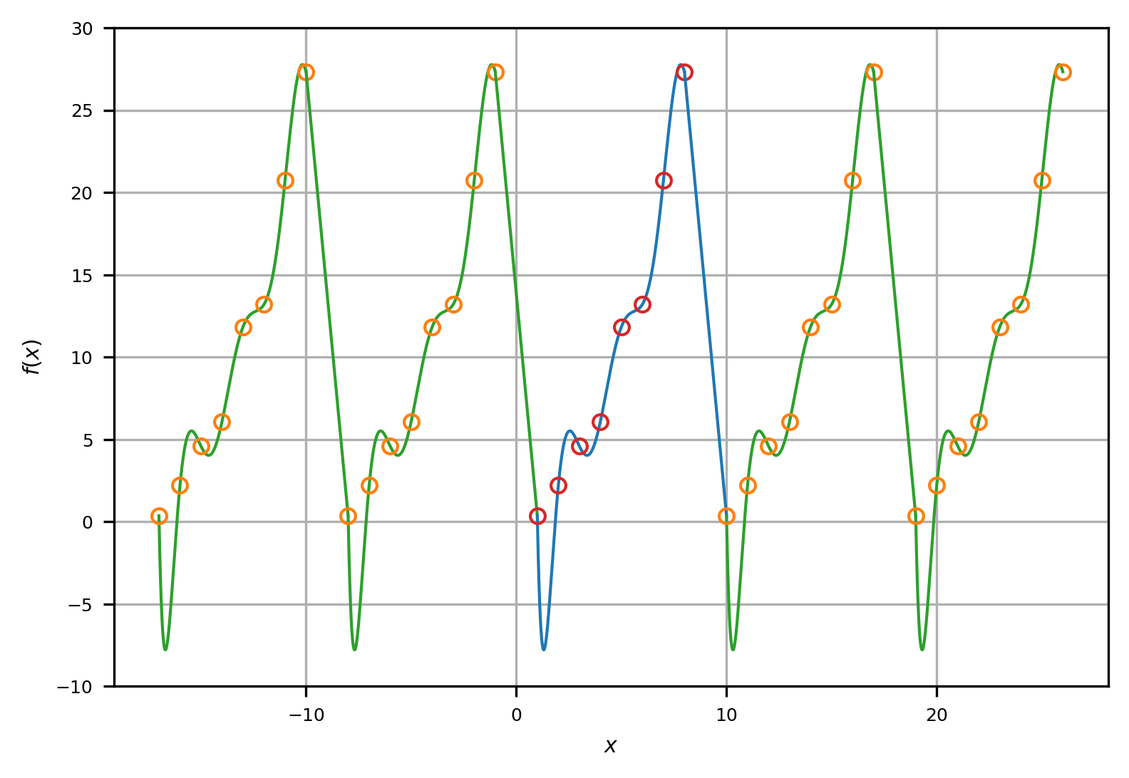
We have got the function looking like a periodic function. But what is the period of our function (the repeated pattern in the plot above)? How long does a single period span in $x$? This is easy. Take a look at the blue part of the curve above which corresponds to one period. We see that this part contains all the points $f_0,f_1,f_2 . . . , f_{N-1}$, but we also need to connect to the adjacent point (from the start of green curve). So, we actually have to include another point in our dataset (to make it periodic) which is given by $f_N = f_0$. This is important to calculate the period. Now, there are in total $N+1$ points with the number of intervals among them as $N$. The interval spacing is $\Delta x$. So, the period is,
\[L = N \Delta x \Delta s=1\]But we usually do not include the last point $f_N$ in the dataset to avoid redundancy (since it simply repeats the $f_0$ value again). We just call our function periodic (in the sense given above) and this is enough.
Now that we got that clarified, the DFT for our data points is given by the strange looking formula:
\[F_k= \frac{1}{N}\sum\limits_{n = 0}^{N-1} f_n e^{-i 2\pi n k/N}\qquad k = -(N/2)+1,..,-2,-1,0,1,2,...,N/2\]We need to understand what this formula says in all its glory. $F_k$’s are the Fourier coefficients and there are in total $N$ of them corresponding to as many Fourier modes. The above formula is actually $N$ similar looking formulas abbreviated into one. The symbol $k$ stands for the wavenumber/frequency associated with the Fourier mode. We will see what this all means in the next post.
P.S.: Have you noticed that the period $L$ does not even appear in this equation?! Have we wasted time in understanding the period of our function (in a strange made-up sense explained above)? NO!! You will later see that it plays a crucial role in understanding the DFT and appears explicitly in the derivative of our function if we are interested in that.
Next article: (In preparation)
Previous article: 1. Fourier transform for confused engineers